Key Takeaways
Here are the 8 best Tableau ETL tools:
1. Hevo Data: Best for no-code data integration and real-time syncing
2. Tableau Prep: Best for preparing and transforming data within the Tableau ecosystem
3. Altair Monarch: Best for extracting and preparing data from legacy sources for Tableau
4. Adverity: Best for data integration and automated reporting with Tableau
5. Microsoft Power Query: Best for data transformation and integration with Microsoft-based tools and Tableau
6. Matillion: Best for cloud-based ETL and transforming large datasets into Tableau-friendly formats
7. Alteryx: Best for advanced data analytics and self-service ETL with Tableau
8. KNIME: Best for building end-to-end data workflows and visualizations for Tableau
Tableau has helped numerous organizations understand their customer data better through their Visual Analytics platform. Data Visualization is the next step after the customer data present in rudimentary form has been cleaned, organized, transformed, and placed in a Data Warehouse. This is where Tableau ETL Tools will come in handy. Integrating ETL tools with Tableau will allow you to load the analysis-ready data from a large number of sources into Tableau after passing through the ETL pipeline.
Here in this article, you will learn about the Tableau ETL Tools in detail. This article will explore the importance of Tableau ETL Tools integration, factors to keep in mind before you decide on a Tableau ETL Tool, and finally, it zeroes in on the best Tableau ETL Tools you choose from to incorporate in yetl tool
our workflow.
Table of Contents
Introduction to Tableau ETL Tools Integration

Despite Tableau’s powerful visualization capabilities, many organizations struggle when handling complex data preparation within the tool itself. Raw business data is rarely visualization-ready. It is scattered across systems, inconsistent in quality, and often requires transformations that slow down dashboards and frustrate end users.
The most effective Tableau strategies follow a clear division of labor: specialized ETL tools handle extraction, cleaning, and transformation, while Tableau focuses on delivering insights through visualization. This separation helps teams achieve:
- Faster dashboard load times
- More reliable and accurate data
- Scalable analytics without overloading Tableau servers
A good starting point is to identify the most resource-heavy preparation tasks and move them upstream into dedicated ETL platforms, allowing Tableau to run at its performance sweet spot.
Hevo is the perfect ETL tool for seamlessly integrating your Tableau data. It automates the data transfer and transformation process to your destination.
This ensures up-to-date dashboards with accurate and real-time data, enhancing your analytics and decision-making capabilities.
Here’s how Hevo can be of help:
- Real-Time Data Synchronization: Updates data in real-time to reflect changes across all systems.
- Error Detection and Handling: Monitors pipelines for errors, providing alerts and automated corrections.
- Automated Data Transformation: Applies consistent rules for data cleaning, normalization, and enrichment.
Join our 2000+ happy customers like Thoughtspot, and Hornblower and empower your data management with us.
Get Started with Hevo at Zero-Cost!Understanding the Top 8 Tableau ETL Tools
 |  | |  |  | |
| Reviews |  4.4 (250+ reviews) | 4.4 (2000+ reviews) | 4.5 (92+ reviews) | 4.4 (240+ reviews) | 4.5 (10+ reviews) |
| Pricing | Hevo: Lorem ipsum dolor sit amet, consectetur adipiscing elit | role-based pricing | Unit-based pricing | Volume-based pricing | Product/service based pricing |
| Free Plan |  Hevo: Free Plan available | | |||
| Free Trial | Hevo: 14-day full-feature free trial | Hevo: Free Plan available | | | |
| Best For | Real-time data pipelines | Native Tableau workflows | PDF/Report data extraction | Marketing data consolidation | Excel/Microsoft environments |
| Tableau Integration | Native Tableau connectors | Built-in integration | Direct Tableau Server export | Custom Tableau dashboards | Power BI to Tableau bridge |
| Pricing (Starting) | $249/month | $70/month | $1995/year | Custom pricing | $10/month |
| Key Strength | No-code automation | Seamless ecosystem | Document processing | Marketing focus | Microsoft ecosystem |
| Data Source Coverage | 150+ sources | Limited to Tableau-supported sources | PDF, text, web, reports | Marketing platforms, digital ads | Excel, web, databases |
| Real-Time Sync | Yes | Limited (batch) | No | Yes (for marketing data) | No |
| Ease of Use | No-code, user-friendly | Drag-and-drop UI | Visual, code-free | UI designed for marketers | Familiar to Excel users |
When you have to deal with complex data preparation, you will need to shift your attention to the available third-party best ETL tool for Tableau to give you what you are looking for. There are a over hundred ETL tools available in the market, that make Tableau ETL integration a worthwhile investment in the long term.
Here you can look at eight key Tableau ETL tools, that will be doing the rounds this year. These Tableau ETL Tools are:
1. Hevo Data

Source: HevoData
Hevo Data is a no-code ETL platform best for business users and small-to-medium teams that need real-time data synchronization into Tableau dashboards without technical complexity. It helps business analysts, marketing teams, and operations managers who want to connect multiple data sources to Tableau quickly while ensuring dashboards always display current information.
Hevo Data makes Tableau integration seamless with its native connectors, automatic schema mapping, and real-time synchronization that remove the burden of manual data preparation. Teams can connect their data sources effortlessly and ensure a smooth flow of information into Tableau.
Unlike traditional ETL platforms that demand technical expertise and constant oversight, Hevo delivers a true no-code experience. Its automatic data formatting keeps Tableau dashboards accurate and always up to date, eliminating the need for ongoing maintenance or manual intervention.
Key Features:
- Real-time Data Synchronization: Automatic refresh ensures dashboards stay current with live business data
- 150+ Pre-built Connectors: Ready-made connections to popular data sources with optimized formatting for seamless integration
- Intelligent Schema Mapping: Smart field mapping automatically translates source data structures into visualization-friendly formats
- Performance Optimization: Data pre-aggregation and indexing are designed to enhance dashboard load times and query performance
- Visual Pipeline Monitoring: Track data flow health with visual alerts and status indicators for complete pipeline visibility


Why Hevo is the Best ETL Tool for Tableau:
Hevo’s architecture is purpose-built for Tableau success, understanding Tableau’s specific data requirements and optimizing every data pipeline accordingly. Unlike generic ETL tools that treat Tableau as just another destination, Hevo’s incremental loading ensures Tableau extracts remain small and fast, while automated data quality checks prevent visualization errors before they reach your dashboards.
With Hevo’s 24/7 monitoring and instant alert system, data teams can maintain reliable Tableau environments without constant manual oversight, making it the most reliable choice for Tableau-centric organizations. This automated reliability, combined with Tableau-specific optimization,s ensures consistent, error-free data pipelines that keep critical business dashboards performing at peak efficiency.
Hevo Data Pricing
- Business: Custom pricing with enterprise-grade Tableau support
- Free: Basic plan at no cost for small data volumes
- Starter: $249/month with full Tableau integration features
2. Tableau Prep

Tableau Prep is Tableau’s native data preparation solution, best for organizations that want seamless integration within the Tableau ecosystem without compatibility issues. It serves data analysts and business users who need to clean, shape, and combine data specifically for Tableau visualization workflows.
Tableau Prep stands out for its zero-friction integration with Tableau Desktop and Server, offering shared authentication, unified metadata management, and direct publishing capabilities. Unlike standalone ETL tools requiring export/import steps, it provides a consistent user experience across the entire Tableau platform with single-vendor support.
Key Features of Tableau Prep
- Data Extraction and Connection.
- Identification of Issues and Errors.
- Understanding your Customer Data (Number of distinct values, data types of fields, number of records, etc).
- Data Enhancement.
- Modification of Data.
- Output Analysis-Ready Data.
This tool houses intuitive drag-and-drop and drop-down menus to visualize your ETL process in Tableau. Tableau Prep allows you to extract data from various data sources:
- MySQL
- Oracle
- PostgreSQL
- Amazon Aurora
- Microsoft SQL Server, to name a few.
Tableau Prep Pricing
The pricing for Tableau Prep is divided into 3 categories:
- Individuals: A single paid plan called Tableau Creator costs $70/user/month billed annually.
- Teams and Organizations: There are 3 sub-plans in place to cater to your needs.
- Tableau Creator: $70/user/month billed annually.
- Tableau Explorer: $35/user/month billed annually.
- Tableau Viewer: $12/user/month billed annually.
- Embedded Analytics: This plan is customizable.
3. Altair Monarch
Altair Monarch is a document intelligence platform best for organizations that need to extract data from unstructured sources like PDFs, legacy reports, and regulatory documents for Tableau analysis. It serves compliance teams and financial analysts who receive critical business data trapped in non-database formats.
Altair Monarch stands out for its automated document parsing capabilities that can identify data patterns in complex documents without manual configuration. Unlike general ETL tools that struggle with unstructured sources, it specializes in converting document-based data into clean, Tableau-ready datasets.
Key features of Altair
- Altair automates time-consuming tasks with the help of repeatable workflows that can be operated without any coding knowledge.
- With Altair, you can combine, clean and export data to tools like Tableau which makes it a key Tableau ETL tool.
- Altair allows you to focus on outliers without losing sight of the bigger picture.
- It also allows users to build their own real-time data monitoring pipelines to track the metrics relevant to their enterprise.
- It further allows you to successfully analyze the impact of alternative responses on future operational performance.
Altair allows you to export to or update the data sources present in Tableau Server. You can do this by providing the necessary information in the sub-tab Server > Tableau Server of the Application Default Settings dialog.
A necessary prerequisite for exporting data to Tableau Server would be the installation of the Tableau TABCMD program. This is a command-line utility that allows users to automate administrative tasks on the Tableau Server site.
With over 80 pre-built data preparation functions, Altair makes the data preparation tasks completely error-free and ensures that more time is spent on data analysis using BI tools like Tableau. This makes Altair a popular choice for an effective Tableau ETL tool.
Altair Monarch Pricing
Altair Monarch costs $1995/user/year for anyone looking for self-service data preparation software.
4. Adverity

Adverity is a marketing-focused data platform best for marketing teams and agencies that need to consolidate campaign data from multiple advertising platforms into unified Tableau dashboards. It serves CMOs and marketing analysts who struggle with fragmented data across Google Ads, Facebook, LinkedIn, and other marketing channels.
Adverity stands out for its pre-built marketing connectors and automated metric calculations that align with common Tableau marketing dashboard templates. Unlike generic ETL tools, it understands marketing data structures and provides campaign-specific transformations that maximize Tableau’s ROI visualization capabilities.
Features of Adverity
- It offers key Marketing operation features like Data Collection, ROI Tracking, Customer Insights, and Multi-User Access.
- It provides the key functionalities of transformation, extraction, loading, and automation.
- The Adverity platform ensures your enterprise keeps up with the latest developments with high scalability.
- It allows the users to build customized dashboards that come with Campaign Insights, Multichannel Tracking, and Brand Optimization to help you get the best out of your data in terms of actionable insights.
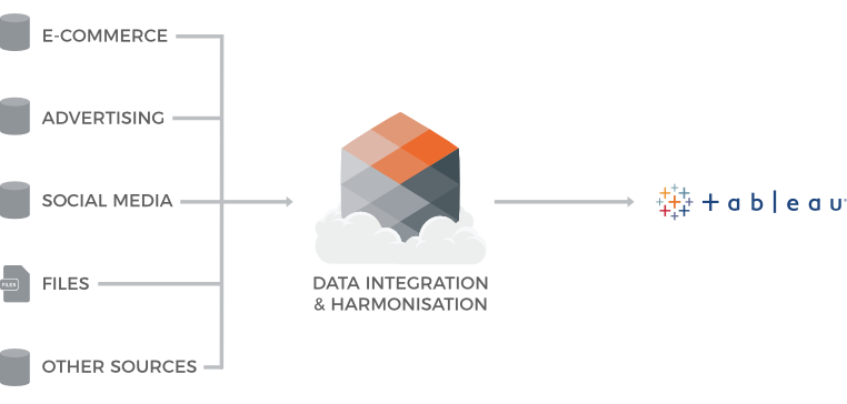
Adverity’s data collection capabilities coupled with a powerful transformation engine allow Tableau users to analyze the customer data on a granular level like never before at a much greater speed.
This integration is highly beneficial as it allows the discovery of actionable insights from high-end data discovery and data visualization capabilities. This integration aims to provide a custom analytics and marketing reporting solution to address the e-commerce and Marketing specific business needs and challenges.
Adverity Pricing
The pricing plans for Adverity are customizable. All you need to do is ask them for a quote and get a pricing plan to fit your budget.
5. Microsoft Power Query

Microsoft Power Query is a data transformation tool best for organizations in the Microsoft ecosystem that need a cost-effective way to prepare Excel and SharePoint data for Tableau visualization. It serves business analysts and Excel power users who want to incorporate Microsoft-based reports into their Tableau workflows.
Power Query stands out for its familiar Excel-like interface and seamless integration with Microsoft data sources, requiring no additional licensing for Office 365 users. Unlike cloud-native ETL platforms, it provides a desktop-based solution that can export transformed data directly to formats that Tableau can consume efficiently.
Key features of Microsoft Power Query
- Power Query allows you to import and work with data from several locations in a single environment by connecting to hundreds of data sources, such as files, databases, online services, and cloud storage systems.
- You can do several data cleansing and modification activities, including filtering, sorting, removing duplicates, splitting columns, merging tables, and more, using its extensive library of built-in transformations.
- Reusable queries are easy to make and save, which will expedite your work and provide consistency throughout workbooks and projects.
- The fundamental features of Power Query are compatible with a number of Microsoft applications, so you can use your transformations across platforms and have a consistent experience.
Microsoft Power Query Pricing
There is a free version and a premium version of Power Query with a free trial available. The paid version begins at $10 per month.
6. Matillion

Matillion is a cloud-native ETL platform best for organizations using cloud data warehouses like Snowflake, Redshift, and BigQuery that want optimal Tableau dashboard performance. It serves data engineers and analysts who need to process large-scale data transformations without moving data out of their cloud warehouse environment.
Matillion stands out for its push-down processing capabilities that execute transformations directly within the data warehouse, resulting in faster Tableau query performance and reduced data movement costs. Unlike traditional ETL tools, it’s purpose-built for cloud architectures and offers native warehouse connectors that maximize Tableau’s cloud deployment benefits.
Some Key features of Matillion
- Browser interface with drag-and-drop functionality. Create complex, potent ETL/ELT tasks.
- Push-down ELT technology processes complicated joins over millions of rows in seconds by using the power of your data warehouse.
- As you construct your ETL/ELT tasks, you may get real-time feedback, validation, and data previews within the application.
- Integrated teamwork. Together, construct occupations in various areas.
- Import/export, server-side undo, and version control.
- You may connect to and get data from more than 80 pre-built connections to well-known web services, in addition to having the option to build your own connector.
Matillion Pricing
There are three price tiers offered by Matillion: basic ($2.00/credit), advanced ($2.50/credit), and enterprise ($2.70/credit). Each tier has a free trial available.
7. Alteryx

Alteryx is an advanced analytics platform best for organizations requiring sophisticated data preparation, predictive modeling, and statistical analysis before Tableau visualization. It serves data scientists and advanced analysts who need to create enhanced datasets with predictive insights and complex data enrichment for Tableau dashboards.
Alteryx stands out for combining ETL capabilities with advanced analytics features like machine learning, spatial analysis, and statistical modeling within a single platform. Unlike basic ETL tools, it enables Tableau users to visualize not just historical data but also predictive insights and statistical correlations that enhance analytical storytelling.
Some Key features of Alteryx
- Regardless of your degree of coding experience, you may utilize either a code-free or code-based interface. You may write code in this interface using the C++, Python, or R languages.
- Alteryx Designer quickly gathers and combines data from several sources, resulting in quicker insights that support more informed decision-making.
- By enabling analytics scalability, repetitive operations may be automated or updated as needed to save time.
- Businesses can choose from a variety of software options offered by Alteryx Designer based on their specific needs. Alteryx Analytics Gallery, Alteryx Analytics Server, Alteryx Connect, and Alteryx Promote are all directly integrated with it. It is also feasible to integrate with R, Python, Tableau, Power BI, SAP, Sharepoint, Salesforce, Github, and Microsoft Azure technologies.
- Using firmographic, geographical, and demographic data for data analysis aids in the production of well-informed business choices.
- The whole analytics workflow may benefit from predictive analytics, and with Alteryx Designer, obtaining, preparing, and modeling data can all be done on one platform. The same might be used to share the outcomes.
Alteryx Pricing
Alteryx begins at $5195.00 per user annually for price. Alteryx offers only one plan, Alteryx Designer, which costs $5195.00 annually per person.
8. KNIME

KNIME is an open-source analytics platform best for organizations with technical teams that want customizable data science workflows feeding into Tableau without licensing costs. It serves data scientists and developers who need flexible, extensible data preparation processes with community-driven innovation.
KNIME stands out for its extensive node library, visual workflow design, and complete customization capabilities through its open-source architecture. Unlike commercial ETL platforms, it offers unlimited scalability and modification options while maintaining full compatibility with Tableau’s data consumption requirements through its active community ecosystem.
Some Key features of KNIME
- Although KNIME Analytics does not come with a business intelligence dashboard functionality, one may create one with the extensive toolkit that is included.
- When it comes to interactive charts for data reporting, KNIME includes several extremely useful ones. These make it possible to manipulate and see individual segments.
- Geo-mapping is one element of KNIME that is quite helpful, especially for direct marketers.
- A set of nodes offered by KNIME can help with predictive analytics. These may be produced as graphs and charts with ease.
KNIME Pricing
Knime starts at $99 for small teams and is free for individual members.

Understanding the Factors to Keep in Mind for Tableau ETL Tools
There are several options available for loading/unifying data in Tableau. These range from built-in Tableau tools/functionalities to user-friendly third-party ETL platforms.
What you would be looking for is the capability of the ETL tool to convert the rudimentary data into a format that is Tableau-friendly.
In this section, you will get a glimpse of a few factors to keep in mind before you decide on an ETL tool to integrate with Tableau for Data Analysis:
- Total Cost of Ownership: You need to keep in mind the budget allocated for acquiring a Tableau ETL tool, the essential functionalities you require in that tool, and the time and money it would take to train your employees to use Tableau ETL tools.
- Technical Knowledge Requirement: You need to look for a Tableau ETL tool that allows you to prepare the data simply. An intuitive tool that lets you understand the functioning in a short period is a major factor that should not be ignored.
- Need for Advanced Capabilities: Pick a Tableau ETL tool that provides essential features like Predictive Modeling, Advanced Mapping, ETL Job Scheduling, and Data Testing. With the advent of technology, a bare-bones Tableau ETL tool wouldn’t suffice your Data Analysis needs in the long run. So you should keep in mind the scale of operations and future capabilities before deciding on the best Tableau ETL tool in the market for you.
- Steps Required for Data Preparation: You should go for a Tableau ETL tool that gives you relevant options for cleaning and preparing the data. For instance, you can use Tableau Desktop for converting data to Tableau date formats, rename fields, and hide unused columns. For more advanced capabilities you can browse through third-party ETL tools to find a Tableau ETL tool that caters to your needs.
- Data Source Requirements: ETL tools can help connect to different types of files like CSV, Excel, or databases and applications. Depending on the sources you rely on for gathering data, pick a Tableau ETL tool that fits your needs.
Benefits of Using ETL with Tableau
- Seamless Integration with Multiple Data Sources: ETL connects Tableau with various data sources for a unified view.
- Improved Data Quality: ETL tools ensure accurate, consistent, and error-free data for reliable insights.
- Handling Large Datasets: ETL tools efficiently process large data volumes, ensuring Tableau performs well with big data.
- Automated Data Workflows: ETL automates extraction, transformation, and loading, saving time and reducing errors.
- Faster Insights: Automated ETL speeds up data preparation, enabling quicker, data-driven decisions.
- Better Data Transformation: ETL tools handle complex transformations, optimizing data for Tableau analysis.
Conclusion
In this article, you have explored the Tableau ETL tools in detail. This exploration included pit stops like the factors determining your choice of the best Tableau ETL tool specific to your use case and a few key Tableau ETL tools to look out for this year.
Extracting complex data from a diverse set of data sources can be a challenging task and this is where Hevo saves the day! Hevo offers a faster way to move data from Databases or SaaS applications into your Data Warehouse to be visualized in a BI tool.
Hevo is fully automated and hence does not require you to code. The Automated data pipeline helps in solving this issue and this is where Hevo comes into the picture. Hevo Data is a No-code Data Pipeline and has awesome 150+ pre-built Integrations that you can choose from. Try a 14-day free trial and experience the feature-rich Hevo suite firsthand. Also, check out our unbeatable pricing to choose the best plan for your organization.
Frequently Asked Questions
1. What is the ETL tool in Tableau?
Tableau Prep is the closest Tableau product to an ETL tool, designed for data preparation and transformation.
2. Which is the best ETL tool?
Depends on your needs; options include Apache NiFi, Talend, Informatica, SSIS, Apache Airflow, Hevo Data, Fivetran, and Stitch.
3. Is Tableau a data extraction tool?
Tableau is primarily a visualization and BI tool, not a dedicated data extraction tool.
Share it with your connections.
-
 Share To LinkedIn
-
 Share To Facebook
-
 Share To X
-
 Copy Link