A Complete Overview of ETL Incremental Loading in 2026

Data doesn’t live in one place. It sits across databases, CRMs, SaaS tools, and internal apps. The whole point of an ETL pipeline is to pull it into a single data warehouse where your team can actually use it, and keep it updated as things change.

The traditional way to do that is a full load: extract everything from the source, load it all into the destination, repeat. When your data is small, this works fine. As it scales into millions of rows, run times stretch, costs climb, and pipelines start falling behind schedule.

Incremental loading fixes this. Instead of moving all your data every time, it moves only what changed since the last run: new rows, updated records, deletions. Your warehouse stays current without the processing overhead or the added cost of shuffling data that hasn’t changed.

In this blog, we cover what ETL incremental loading is, how it works, the methods to implement it, and the challenges you’ll run into, along with ways to handle them.

What is ETL Incremental Loading?

ETL incremental loading transfers only newly added or modified data from source to destination, rather than reloading the entire dataset on every run.

Most ETL pipelines run on a schedule. Each time they fire, they need to bring the destination in sync with what changed in the source. Incremental loading does this by identifying what’s new or different since the last run and moving only that. The smaller that change set, the faster and cheaper the run.

• By default, incremental loading is time-based: it filters source records by when they were created or modified, using a column like created_at or updated_at
• It uses a reference point called a high-water mark to know where the last successful load ended and where the next one should begin
• Unlike full loads, which copy the entire source table every run, an incremental load only touches a fraction of the data
• It preserves historical records in the destination even when the source system has already deleted them

Key components of ETL incremental loading

1. Source change detection

The pipeline needs to know which records changed since the last run. This is determined by a timestamp column, an auto-incrementing ID, or the database transaction log. 

Without a clear detection method, the pipeline either moves the wrong data or misses records.

2. Extraction process

Only records that meet the change criteria get pulled. If you’re using timestamps, that means rows where updated_at is greater than the last run time. If you’re using IDs, it’s everything above the last processed ID. The rest of the table stays untouched.

3. Transformation logic

Extracted records may need reformatting before they load. Column types, field names, and business rules often differ between source and destination. Transformation applies those mappings before the data reaches the target.

4. Loading mechanisms

Two options: stream or batch. Stream processes records as they arrive, suited for small, continuous changes. Batch groups updates and loads them on a schedule, better for large volumes. The right choice depends on how current the data needs to be.

5. Data validation and consistency checks

After loading, compare row counts and checksums between source and destination. If a record was skipped or a batch only partially loaded, this is how you catch it. Without these checks, bad data can sit in the warehouse for days before anyone notices.

Why do you need ETL incremental loading?

1. Faster Processing

It usually runs much faster because there is less data to interact with. Considering there are no bottlenecks, the time it takes to transfer and transform data is directly related to the amount of data involved. In many cases, interacting with half the data will reduce the execution time by the same amount. 

2. Better Risk Handling

The lesser amount of data to touch reduces any potential surface risk associated with a particular load. Sometimes, a given loading process may fail or malfunction, leaving the target data inconsistent. The incremental loading technique is a fractional loading method. 

It reduces the amount of data you add or change, which may need to be rectified in the event of any irregularity. Because less data is reviewed, it also takes less time to validate the data and review changes.

3. Consistent Performance

With ETL Incremental Loading, you get constant performance despite any fluctuating workloads. Generally, today’s load always contains more data than yesterday’s. Therefore, running a full load can be a time-consuming method as the time required for processing increases monotonously. 

It only transfers data in case of any modifications, increasing the likelihood of more consistent performance.

4. Recording Historical Data

You will notice that many of the source systems regularly delete old data. This can be problematic, as often you may be required to report this data to your downstream systems. Using the ETL Incremental Loading process, you will need to load only the new and modified data. 

This allows you to keep all the source data(including the data deleted from the upstream sources) in your target destination system.

Difference between ETL full loading and ETL incremental loading

Parameter	ETL Full Loading	ETL Incremental Loading
Data loaded	Entire dataset, every run	Only new or modified records since the last run
Speed	Slower — processes all rows regardless of changes	Faster — only touches a fraction of the data
Resource usage	High — heavy on compute, memory, and I/O	Low — resources scale with the volume of changes
Network load	High — transfers the full dataset each time	Low — transfers only what changed
Cost	Higher — more compute and storage cycles per run	Lower — fewer resources consumed per run
Complexity	Simple to set up and maintain	More complex — requires change tracking logic
Error handling	Easy — redo the entire load from scratch	Harder — requires sequential loading; errors can cascade
Techniques required	None	Timestamps, sequential IDs, CDC, or row hashing
Historical data retention	Overwrites previous data; older records can be lost	Retains history in the destination even if the source deletes it
Loading frequency	Typically less frequent — nightly or weekly	Can run frequently, including near real-time
Best for	Small datasets, initial loads, or infrequent refreshes	Large, frequently updated datasets

When should you use ETL Incremental Loading?

ETL Incremental Loading is an excellent alternative to ETL Full Loading in the following cases:

• Dealing with a comparatively bigger data source
• Facing slower performance issues while querying data due to data size and technical limitations.
• Tracking the data changes is possible.
• In several data sources, old data gets deleted. You might want to retain that deleted data in the target system, such as a Data Warehouse.  

Incremental Load Method for Loading Data Warehouse Example 

• To understand the working of the ETL Incremental Loading, you can consider a data source having 2 tables, i.e, sales and customer. 

Customer Table

CustomerID  CustomerName  Type         Entry Date
1           Jack          Individual   11-Apr-2021
2           Roland        Individual   11-Apr-2021
3           Bayes          Corporate   12-Apr-2021

Sales Table

ID         CustomerID    ProductDescription   Qty   Revenue  Sales Date
1          1             Chart Paper          100    4.00    11-Apr-2021
2          1             Board Pin (Box)      1      2.50    11-Apr-2021
3          2             Permanent Marker     1      2.00    11-Apr-2021
4          3             Eraser       	      200   75.00    12-Apr-2021
5          1             Pencil (HB)          12     4.00    12-Apr-2021

• Using ETL Incremental Loading, 2 records from the “Customer Table” and 3 records from the “Sales Date” table will be uploaded to your target data warehouse on 11 April 2021. Now, on the next day (12 April 2021), only 1 record from the customer table and 2 records from the sales table are uploaded to your destination system.
• This is because it only uploads the newly created or modified records instead of copying the entire table.
• To know which records are already present in the target data warehouse, you can use the Entry data column of the customer table and the Sales Data column of the sales table.
• You can now record the date till which the data is present after the data is loaded on that day and then only upload data with the date greater than the previously recorded date. You can create a table “batchdate” to store these dates.

Batch_ID  Loaded_Until  Status
1         11-Apr-2021   Success
2         12-Apr-2021   Success

You can now write your respective SQL Queries to extract data from the: 

Customer Table 

SELECT c.* 
FROM Customer c
WHERE c.entry_date > (select nvl(
    max(bd.loaded_until), 
    to_date('01-01-1900', 'MM-DD-YYYY')
  )
from batchdate bd
where bd.status = 'Success'
);

Sales Table

SELECT s.* 
FROM Sales s
WHERE s.sales_date > ( select nvl(
    max(bd.loaded_until), 
    to_date('01-01-1900', 'MM-DD-YYYY')
  )
from batchdate bd
where bd.status = 'Success'
);

• Initially, no data has been loaded, so the batchdate table will be empty. Hence, when you execute the above queries, the nvl function will give the date 01-01-1900 as the max(bd.loaded_until) will return a NULL value.
• This means everything will be extracted. After loading the data for April 11, the first entry can be made into the batchdate table. For the next day(April 12), the max(bd.loaded_until) will now return April 11, 2021. Hence, the data only after April 11 will now be uploaded to the data warehouse.

How to implement ETL incremental loading

When choosing the ideal methods of incremental loading in data warehouse settings, it’s essential to consider the source systems, the volume of data to be updated, and the needed load frequency.

To effectively implement the ETL Incremental Loading for your use case, you can through the following two methods:

• Method 1: Destination Change Comparison
• Method 2: Source Change Identification

Method 1: Destination Change Comparison

This method requires a row-wise analysis to compare the unchanged data and the data that has been newly added or modified. Hence, this process might perform slower than the source change Identification method.

This technique requires you to bring all the data you need to monitor for changes into the ETL Data Pipeline. Compared to the Source Change method, it has fewer assumptions. Owing to its flexibility, it can work for almost any structured data source, including text files, XML, API result sets, and other non-relational structures.

You can use this method via the following approaches: 

• Brute Force
• Row Hash
• Upsert Operations

1.1: Brute Force

This is the most direct way & with the least ETL requirements to use the destination change comparison method by analyzing the data row-by-row. If no other comparison method is available, the Brute force comparison works. If you can not use other methods, use it as a last resort. 

1.2: Row Hash

For Row hashes, you will be using a single column that stores a kind of calculated binary version of the column used for comparison. This hashed binary value is a computed aggregate of all the specified columns.

Unlike the traditional method of manually comparing each column, Row hashes are usually more efficient. However,  the hash value needs to be calculated, which adds a bit of complexity and overhead but is usually worth improving performance.

1.3: Upsert Operations

UPSERT, i.e., update & insert, will effectively process both newly added and modified data in one step. This is done by matching the unique key columns and comparing the ones confirming the change. You can also bring in the row hash method within this merge operation to make the comparison.

Popular RDMS systems such as SQL Server, Oracle, Postgres, and MySQL work with the UPSERT logic. On most systems, UPSERT operations can also handle data deleted at the source. You can also decide whether to delete the data on the target or softly delete it, i.e., leave it as it is and mark it as deleted.

Method 2: Source Change Identification

This method opts for a selective approach by extracting only the new and modified data from the source system since the last run of the loading process. This essentially puts a limit on the amount of data that is being brought to the ETL Data Pipeline.

It is done by only extracting the data that actually needs to be moved and excluding the unchanged data from the load cycle. The less data you need to interact with, the faster the data processing. To apply this technique, you can employ the following approaches:

• Change Tracking
• Update Dates or Row-level Insert
• Change Data Capture

2.1: Change Tracking

For a simple, reliable & easy-to-use method, you can try out the change tracking technique present in most of the RDBMSs today. Change tracking makes it easy to see which rows have been newly created, modified, or deleted since the last load. However, this is not always an option because you need to modify the source database to use change tracking for incremental loads. 

2.2: Update Dates or Row-level Insert

This is the easiest way to detect changes in the source. With this method, for each table, you will have a column that records the date the data was loaded and the date the data was modified. This allows you to identify each row when it changes effectively. Although it turns out that this method can be unreliable.  Especially on third-party systems that you can’t control. 

2.3: Change Data Capture

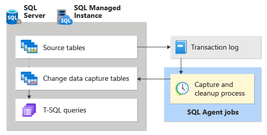
Change data capture is another brilliant source-side change detection method available in SQL Server and other RDBMS systems. Though change data capture allows you to perform several tasks compared to simple change detection, it can still be used to identify which data has been newly created, modified, or deleted.

2.4: With a ‘Last Updated Timestamp’

The source system includes a column called ‘Last Updated Timestamp’, which indicates the last time each row was modified. By leveraging this column, we can selectively extract updated records after the last extraction timestamp. 

For example, if the previous load was completed on 2022-01-09 12:00:00, in the next run, we would only extract records where the ‘Last Updated Timestamp’ is later than this timestamp. This method allows us to track both new records and updates.

2.5: Without a ‘Last Updated Timestamp’

When there is no ‘Last Updated Timestamp,’ a control table can be used to store metadata like the last extraction timestamp and the number of loaded records. A surrogate key or a combination of natural keys with a checksum can be used to identify new or changed records. Using an auto-incrementing ID for new records is another common approach to track new records. However, tracking updated records with this approach is not possible.

Example: 

Consider a large-scale e-commerce platform as an example. Suppose the platform operates a ‘users’ table that maintains a record of all users, with new users registering every second.

Using a Full Load strategy would entail loading the entire ‘users’ table into the data warehouse during each ETL run, despite the majority of the data remaining unchanged. This approach would be highly inefficient, given the size of the table. 

Alternatively, an Incremental Load strategy would only load new users since the previous ETL run. The process is straightforward if a ‘Last Updated Timestamp’ exists in the ‘users’ table. However, if not, the ‘user_id’ (assuming it is an auto-incrementing ID) can be used, and the highest ‘user_id’ loaded can be stored in the control table. During the subsequent ETL run, only users with a ‘user_id’ greater than the stored value would be extracted.

What are the key challenges of ETL incremental loading?

1. Monitoring

While extracting and consolidating data from different sources, errors will come up. Expired API credentials, connectivity issues, and schema mismatches cause silent failures or partial loads that are easy to miss.

To manage this, set up automated alerts on pipeline runs rather than relying on manual checks. Most ETL tools log run status, row counts, and error types. Use those logs to build threshold-based alerts: if row counts drop significantly between runs without a clear reason, something went wrong. Catching it early is the difference between a quick fix and a downstream data quality issue.

2. Incompatibilities

Adding new records that conflict with existing data, for example, writing an integer to a column expecting text, creates bottlenecks. End users querying that data get inaccurate or incomplete results, and new records can’t be added until the conflict is resolved.

Use ETL tools like Hevo, which has automatic schema detection to handle this. They can adapt when a source column changes type or a new field appears, adjusting the mapping before the data hits the destination. For custom pipelines, validate data types before loading and route non-conforming records to a staging table for review rather than letting them break the pipeline.

3. Sequencing

Distributed pipelines process records in parallel, which means data can arrive at the destination out of order. This gets particularly messy when records are being modified or deleted.

Design your pipeline to handle records idempotently — the same record can be applied multiple times without corrupting the output. Upserts handle this well. For cases where strict ordering matters, add a sequence number or event timestamp to each record and sort before loading.

4. Dependencies

Pipelines are rarely isolated. One table often depends on another finishing first. If process 1 fails, running process 2 on stale data creates compounding problems, and the more tables you add, the worse this gets.

Map dependencies explicitly in your orchestration layer. Tools like Apache Airflow, Prefect, or dbt let you define execution order using DAGs. Set clear failure policies for each process: fail fast, skip, or retry, and document which downstream tables depend on which upstream loads.

5. Tuning

Keeping data accurate and consistent in the destination requires ongoing attention. Run times drift, source schemas change, and edge cases surface over time. Treating tuning as a one-time task means problems accumulate quietly.

Build reconciliation checks directly into the pipeline: compare row counts, sums on key metrics, and record counts between source and destination after each load. If something is off, the pipeline flags it automatically. Treat this as regular maintenance, not a fix for when things break.

How Hevo helps you implement incremental loading

Setting up incremental loading from scratch means writing extraction logic, managing state, handling schema changes, and building monitoring for every source. Hevo handles all of that out of the box across 150+ data sources, so you can focus on using the data instead of maintaining the pipeline.

When you connect a source, Hevo identifies the right change detection method automatically depending on what the source supports. For databases like MySQL, PostgreSQL, and MongoDB, Hevo reads directly from the transaction log. That means every insert, update, and delete gets captured in real time, including deletions that timestamp-based methods miss entirely.

Beyond extraction, here is what Hevo manages for you:

• No-code setup: Connecting a source, configuring incremental sync, and setting frequency takes minutes, no custom scripts, no infrastructure to manage
• Automatic schema detection: When a source column changes type or a new field is added, Hevo detects it and updates the destination mapping — pipelines don’t break when schemas evolve
• Real-time replication: Changes move from source to destination as they happen, not on a fixed overnight schedule
• Built-in monitoring: Every run is logged with row counts, error details, and load status so issues surface before they affect downstream reporting

Conclusion

In this article, you have learned in detail about the ETL Incremental Loading process. Compared to the Full Loading process, incremental loading is fast, can perform consistently with fluctuating workloads, and allows you to store historical data. You can implement change detection methods using either source- or destination-sided methods.

As you collect and manage your data across several applications and databases in your business, it is important to consolidate it for a complete performance analysis of your business. However, it is a time-consuming and resource-intensive task to continuously monitor the Data Connectors. To achieve this efficiently, you need to assign a portion of your engineering bandwidth to integrate data from all sources, Clean & Transform it, and finally, Incrementally Load it to a Cloud Data Warehouse or a destination of your choice for further Business Analytics. 

All of these challenges can be comfortably solved by a Cloud-based ETL tool such as Hevo Data. Sign up for a 14-day free trial and simplify your data integration process. Check out the pricing details to understand which plan fulfills all your business needs.

Frequently Asked Questions