Working with AWS DataBrew: 3 Easy Steps

Data is essential for business growth in today’s competitive world. Access to high-quality data gives companies an edge, but cleaning and managing raw data from multiple sources can be time-consuming. This process turns low-quality data into valuable insights for analysis, machine learning models, and BI tools.

With AWS DataBrew, you can automate data preparation. This tool helps data scientists and analysts quickly clean and normalize raw data using pre-built transformations. AWS Glue DataBrew saves you time, so you can focus more on analyzing data.

In this article, we’ll explore how AWS DataBrew works and walk through the steps to create a sample dataset, cleaning and normalizing it efficiently.

What is AWS DataBrew?

AWS DataBrew is a serverless data preparation tool that helps companies, data scientists, and analysts clean and normalize data without coding. It reduces data preparation time by up to 80% using machine learning. With over 250 pre-built transformations, it automates tasks like filtering anomalies, correcting invalid values, and standardizing data. DataBrew offers an interactive interface to easily discover, visualize, and clean raw data, enabling users to handle terabytes of data efficiently.

Key Features of AWS DataBrew

Some of the main features of AWS DataBrew are listed below:

• Visual Interface: AWS DataBrew comes with an interactive visual interface that makes it easier for users to clean and prepare the raw data using the click and select feature.
• Automate: AWS DataBrew offers may save transformations that users can use to directly apply transformations for cleaning and normalizing data.
• Map Data Lineage: With the help of AWS Glue DataBrew, users can visually map the lineage of data to understand the data sources and their transformations steps.

What is AWS Glue?

It can take a long time to create a workflow that efficiently accomplishes the above-mentioned operations. This is where AWS Glue comes into play. It’s a fully managed ETL solution that’s built to deal with massive amounts of data. Its task is to harvest data from a variety of different AWS services and integrate it into data lakes and warehouses. Since it offers both code-based and visual interfaces, Glue is extremely versatile and simple to use.

AWS DataBrew is a popular and recent feature. DataBrew data can be cleaned, normalized, and even augmented with Glue without having to write any code, and Glue Elastic Views makes merging and replicating data across disparate data stores with SQL a breeze.

Want to know how to build an AWS Glue S3 pipeline from scratch? Read our blog to learn more about it.

Working of AWS DataBrew

Let’s first understand how AWS DataBrew works and helps in quickly preparing data. The following steps to prepare data using AWS DataBrew are given below:

• You can connect one or more Datasets from AWS S3, AWS Redshift, RDS, and AWS Glue Data Catalog or upload the file from your local system from the AWS DataBrew Console that supports CSV, JSON, Parquet, and .XLSX formats.
• Then, create a project so that you can visually explore, understand, analyze, clean, normalize the data from the Dataset. 
• By visualizing all the information you can quickly identify patterns in the data and spot anomalies.
• After that, you can generate a data profile of the Dataset with over 40 statistics by running a job in the “Profile View”.
• AWS DataBrew will give you recommendations to improve the data quality. It can help you with cleaning data using more than 250 pre-built transformations.
• You can save, publish and version recipes. After that, you can automate the data preparation tasks by applying recipes to all incoming data.
• You can visually track and explore the connectivity of Datasets with projects, recipes, and jobs.

Preparing a Sample Dataset with AWS DataBrew

Now that you have understood about AWS DataBrew. In this section, you will go through the process to create a sample dataset using AWS DataBrew. The simple steps for using AWS DataBrew are listed below:

• Step 1: Connecting to a Dataset
• Step 2: Exploring the Dataset
• Step 3: Applying Transformations Using AWS DataBrew

Step 1: Connecting to a Dataset

• Log in to your AWS Glue DataBrew Console here.
• Create a new project by navigating to the “Projects” tab and then clicking on the “Create project” option.
• You can enter any name to the project. In this tutorial, the project name is “Comments”, as shown in the image below.

• Along with this, a new recipe will also be created and automatically updated with the data transformations that you will see further in this tutorial to AWS DataBrew.
• Then, select the “New Dataset” option and name it as you like, eg.- “Comments”, as shown in the image below.

• Now, the new dialog box will ask you to connect to a new Dataset. Here, you need to upload the new Dataset that you want to use.
• For this tutorial, the “Comments.csv” file is used as a Dataset. While working with real Datasets, you need to connect AWS DataBrew with AWS S3 or an existing source in the AWS Glue Data Catalog.
• Next, for the “Comments.csv” file, you can provide the AWS S3 destination to store the Dataset file, as shown in the image below.

• The “Comments.csv” file contains the first column as the name of the columns and rests all the rows have the values that include comments, category, customer id, and item id as text, rating as numerical, and comment_sentiment and support_needed.
• The sample data is shown below.

customer_id,item_id,category,rating,comment,comment_sentiment,support_needed
234,2345,"Electronics;Computer", 5,"I love this!",Positive,False
321,5432,"Home;Furniture",1,"I can't make this work... Help, please!!!",negative,true
123,3245,"Electronics;Photography",3,"It works. But I'd like to do more",,True
543,2345,"Electronics;Computer",4,"Very nice, it's going well",Positive,False
786,4536,"Home;Kitchen",5,"I really love it!",positive,false
567,5432,"Home;Furniture",1,"I doesn't work :-(",negative,true
897,4536,"Home;Kitchen",3,"It seems OK...",,True
476,3245,"Electronics;Photography",4,"Let me say this is nice!",positive,false

• Now, it will ask you for permissions and select the role to access AWS DataBrew.
• In the “Access Permissions” select the AWS Identity and Access Management (IAM) that will grant the permissions to access data to AWS S3. 
• Here, select the “Role name” as the “AWSRoleForDataBrew” option from the drop-down menu, as shown in the image below.

Step 2: Exploring the Dataset

• If the dataset you are using is big then you can use the “Sampling” technique to limit the number of rows. 
• You will make use of projects to create recipes and then jobs to apply these recipes to all the data. 
• You can use the “Tagging” to manage, filter, and search resources that you created with the help of AWS DataBrew, as shown in the image below.

• After, setting all these configurations, the project will start preparing and exploring the dataset.
• Once the data preparation is done, it will show you the default Grid View where it will show you a summary of each column having range values and statistical distribution having numerical columns.
• You can change the view by selecting Schema View to drill down on the schema and Profile View to collect statistical summaries about the data which is useful for large datasets.
• Once the job is done, you can apply exploratory Data Analysis to the data by identifying the correlation between columns, gathering summaries and how many rows and columns are valid. AWS DataBrew presents all this information visually to help you easily identify the patterns in data, as shown in the image below.

• You can even drill down into a specific column after selecting it.

Step 3: Applying Transformations Using AWS DataBrew

• Now let’s explore the “category” column. Here, it contains two pieces of information, separated by semicolons. 
• For example, you can view the data in the first row as “Electronics;Computers”. 
• You can split the “category” column into two different columns by selecting the “category” column then clicking the three dots option to explore more options.
• Here, select the “Split Columns” option and then further select the “On a single delimiter” option, as shown in the image below. 

• This will divide the “category” column into two separate columns with column names “category_1” and “category_2”. You can rename these columns as per your choice. For example – renaming them to “category” and “subcategory”.
• Similar changes will be made to other categories.
• Next, let’s move to the other column “rating” which contains the numeric values between 1 and 5. You can rescale these values using “min-max normalization” so that all the values are rescaled between 0 and 1. You can also use many other advanced techniques and a new column with the name “rating_normalized” will be added.
• Similarly, you can use other transformation techniques on different columns to make optimize the data for Analysis using Machine Learning models. You can use a few common techniques such as one-hot encoding, missing values, word tokenization, etc. based on the type of data.
• Once your data is ready, it can be published and used in a recurring job processing similar data, as shown in the image below.

• The recipe contains a list of all the transformations that are to be applied and the while the job is running the output will store in the AWS S3.
• The output data is available for Data Analytics, feeding it to Machine LEandig models, building reports, and feeding it to BI tools for Visualization, as shown in the image below.

That’s it! You have completed the process to create a sample Dataset using AWS DataBrew and understood different transformation techniques and how AWS Glue DataBrew helps you quickly prepare data, clean and normalize it.

AWS DataBrew vs SageMaker DataWrangler

AWS DataBrew vs SageMaker DataWrangler: Both services were released around the same time and serve a similar purpose, making it a tough choice for users, especially Data Scientists.

Who’s it for?:

• DataWrangler: Tailored for advanced users like data scientists, offering custom transformations and quick machine learning model creation. It’s great for high-level data analysis and feature tracking.
• DataBrew: Ideal for users who need simplicity and ease. It comes with many built-in transformations and doesn’t require deep technical knowledge, making it accessible to a broader audience.

Flexibility vs Simplicity:

• DataWrangler provides more flexibility but requires technical expertise.
• DataBrew simplifies the process, covering most user needs without the need for in-depth technical understanding.

Who should use which?:

• DataWrangler is perfect for Data Scientists working on custom data processing for machine learning.
• DataBrew is better for those who prefer a straightforward, no-fuss approach to data preparation.

Conclusion: Both tools have distinct target audiences. DataWrangler is for those needing advanced features, while DataBrew focuses on simplicity for the majority of users.

AWS DataBrew Example

Step 1: Creating a Source of Data

The creation of an S3 bucket is a step in this example that isn’t directly related to DataBrew. Go to the AWS S3 Management Console and click “Create bucket” to create an S3 bucket.

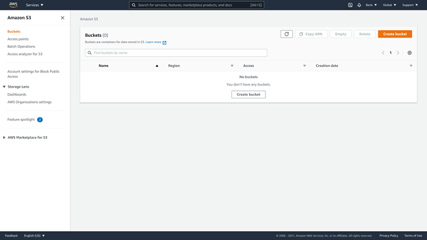
Make a new bucket called “edlitera-databrew-bucket” and label it such. All other possibilities should be left alone.
The bucket will appear on our AWS S3 interface once you’ve created it.
You’re ready to work with DataBrew now that you’ve created a bucket. Click on the datasets tab on the DataBrew page, then “Connect new dataset.” When connecting a new dataset, there are a few factors to consider:

• Name of the data set
• source of data
• Tags for the output destination (optional)

You can call this dataset “wine-reviews” and choose “File upload.” You may select a dataset on the local system and instruct AWS DataBrew to send it to the empty bucket you generated earlier using file upload. The new dataset should be ready to use now.

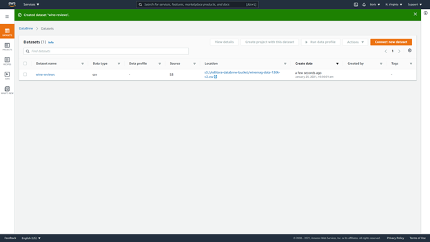
Step 2: Data Analysis

Let’s start with some basic data analysis after you’ve defined the dataset that you’ll be using. A dataset profiling feature is included in AWS DataBrew. When working with data that is foreign to you, profiling data can be very valuable. You must go to the “Jobs” menu to create a profile job. Three possibilities will be presented to you:

• Recipe jobs
• Profile jobs
• Schedules

At this time, you’d like to develop a profile of your dataset in order to get a better understanding of how your data appears. Select the “Profile jobs” tab and then “Create job” from the drop-down menu.

You’ll need to enter values for the following parameters when defining the job:

• Job name
• Job type
• Job input
• Job output settings
• Permissions 
• Optional settings

Your job title will be “wine-review-profile.” You’ll pick that you want to make a profile job and then your dataset. You’ll use the bucket you generated earlier for output.

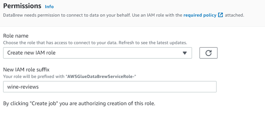
Finally, you must establish a role. You’ll establish a new role called “edlitera-profiling-job” because you don’t have one to choose from yet.
You only need to click “Create and run job” after you’ve defined everything, and AWS DataBrew will begin profiling your dataset.
When the job is finished, you can go to the upper right corner and click “View profile.”

The following sections make up a dataset profile:

• Dataset preview
• Data profile overview
• Column statistics
• Data lineage

The “Dataset preview” section shows the dataset together with details like the dataset name, data size, and where our data is housed, among other things.

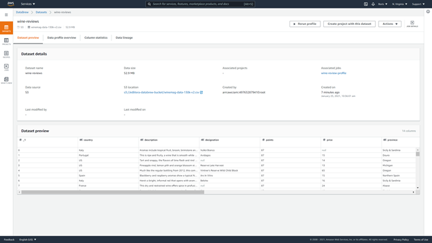
The “data profile” shows details about:

• Number of rows
• Number of columns
• Data types of columns
• Missing data
• Duplicate data
• Correlation matrix

There are no duplicates in your dataset, although it is lacking certain information. You may assume that you have a number of columns with categorical data because the correlation matrix only shows three values and you have fourteen columns in total, which is also corroborated by the data types section.

The following information is displayed when you click on “column statistics“:

• Column data type
• Percentage of missing data in column
• Cardinality
• Value distribution graph
• Skewness factor
• Kurtosis
• Top ten most frequent unique values 
• The correlation coefficient between columns

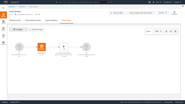
Finally, the “Data lineage” page displays a visual representation of our data’s lineage.

Step 3: Data Transformation

As previously said, this is most likely AWS DataBrew’s most significant feature. A transformation recipe, or a series of transformations defined in a reusable format, is used to transform a dataset. You’ll create a DataBrew project and define a DataBrew transformation recipe to demonstrate some of the features DataBrew has to offer.

To do so, go to the “Projects” menu and click on “Create project.”
You must define values for the following variables in order to create a project:

• Project name
• Recipe name 
• Dataset
• Permissions
• Sampling and tags (optional)

Your project will be called “wine-reviews-transformation,” and your new recipe will be called “wine-reviews-transformation-recipe.” After that, you’ll select “wine-reviews” as the dataset you wish to work with.

You’ll leave the option for “Sampling” at default, which means you’ll look at a sample of 500 rows, which is adequate to show how recipes are made. To complete the process definition, you’ll utilize the same role as before: the “AWSGlueDataBrewServiceRole-wine-reviews” role.

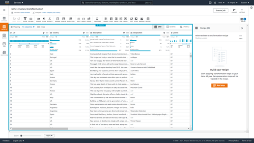
AWS DataBrew will then begin the process of preparing a session, which will take some time. Your data can be shown as a grid or a schema. You’ll show it as a grid for this demonstration.

It’s time to get to work on your recipe. When you pick “Add step” from the drop-down menu, you can choose a transformation to apply to your dataset. In the toolbar above your dataset, you can see the many changes you can execute. They are used for a variety of reasons.

AWS DataBrew: Pros & Cons

• Connect data straight from your data lake, data warehouses, and databases to evaluate the quality of your data by profiling it to understand data patterns and find abnormalities.
• With an interactive, point-and-click visual interface, choose from over 250 built-in transformations to visualise, clean, and normalise your data.
• Visualize your Data’s Lineage to better understand the numerous data sources and transformation procedures it has gone through.
• Apply previous transformations immediately to new data as it enters your source system to automate data cleaning and normalisation procedures.
• Your dataset’s first 20,000 rows are used to create a data profile. It took 2 minutes and 2 seconds to complete this task. This report will not appear if your data becomes erratic after row 20k. This is merely a cursory examination, not a comprehensive analysis.
• Correlations will be offered for your numerical data. This issn’t particularly amazing if you have largely strings.

AWS DataBrew: Best Practices

One-Hot a categorical column

When preparing data for machine learning, setting up One-Hot columns for a multi-category column is a regular activity. To execute this operation, you can utilise one of several Python modules. It was even easier to use this interface. There appear to be some limits to this technology that it may not be able to overcome. (For the sample dataset, there were more than ten categories.)

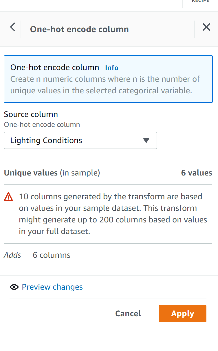
Press the Apply button. New columns appear out of nowhere. That’s all there is to it.

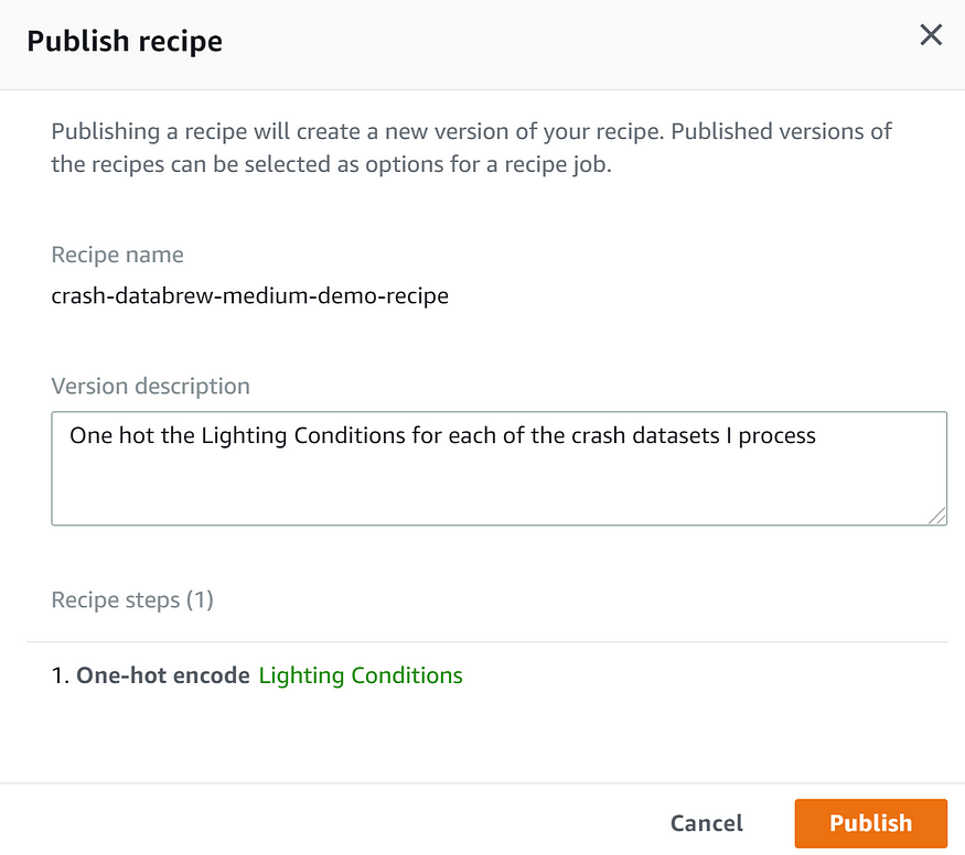
Publish your recipe

Make your recipe public so that others can benefit from it.

AWS DataBrew: Pricing

Cost is always a factor to consider. Each interactive session costs $1.00. Transformation jobs cost $0.48 per node hour. The coolest aspect is that it’s completely pay-per-use. As a result, even the casual enthusiast will find the tool highly accessible and affordable.

Conclusion

In this article, you learnt about AWS Glue DataBrew and the working of this tool that help in automating the data preparation tasks and saves time. You also went through the process to create a sample Dataset using AWS DataBrew and understood how to use AWS Glue DataBrew for cleaning, normalizing, and preparing data with 250 pre-built transformations, automation, and visual interface to quickly identify the patterns in data.

Amazon Redshift and Amazon S3 stores data from multiple sources and every source follows a different schema. Instead of manually writing scripts for every source to perform the ETL (Extract Transform Load) process, one can automate the whole process. Hevo Data is a No-code Data pipeline solution that can help you transfer data from 150+ sources to Amazon Redshift, S3, or other Data Warehouse of your choice. Its fault-tolerant and user-friendly architecture fully automates the process of loading and transforming data to destination without writing a single line of code. 

Want to take Hevo for a spin? Sign Up here for a 14-day free trial and experience the feature-rich Hevo suite first hand.

Share your experience of learning about the AWS DataBrew in the comments section below!

FAQs